

This guide explains how bathymetry contour data from Kartverket can be converted into a continuous 3D seabed model using QGIS.
The workflow transforms depth contours into a raster elevation model representing seabed morphology, suitable for visualization and spatial understanding in tools such as Blender or digital twin environments
A continuous 3D seabed model exported as a GeoTIFF DEM, with an optional heightmap suitable for 3D visualization and displacement workflows.
Example visualization:
View interactive 3D seabed example →
⚠️ Intended Use and Disclaimer
The workflow described in this article is intended exclusively for visualization, conceptual analysis, and general spatial understanding of seabed conditions. Generated 3D models must not be used for navigation, marine operations, engineering decisions, dredging planning, construction activities, or safety-critical assessments. The produced models do not replace hydrographic surveys, certified nautical charts, or officially approved depth measurements. PORT360 assumes no responsibility for operational decisions made based on models generated using this workflow.
Step 1 — Create a Working Area (Project Extent)
Creating a dedicated working-area polygon ensures that all exported datasets share the exact same spatial extent. This guarantees alignment between:
- heightmaps
- textures
- shapefiles
- GeoJSON exports
- 3D models
Create Shapefile Layer
Layer → Create Layer → New Shapefile Layer
Settings:
- Geometry type: Polygon
- CRS: EPSG:25835 — ETRS89 / UTM Zone 35N
- Name example: Extent-locations.shp
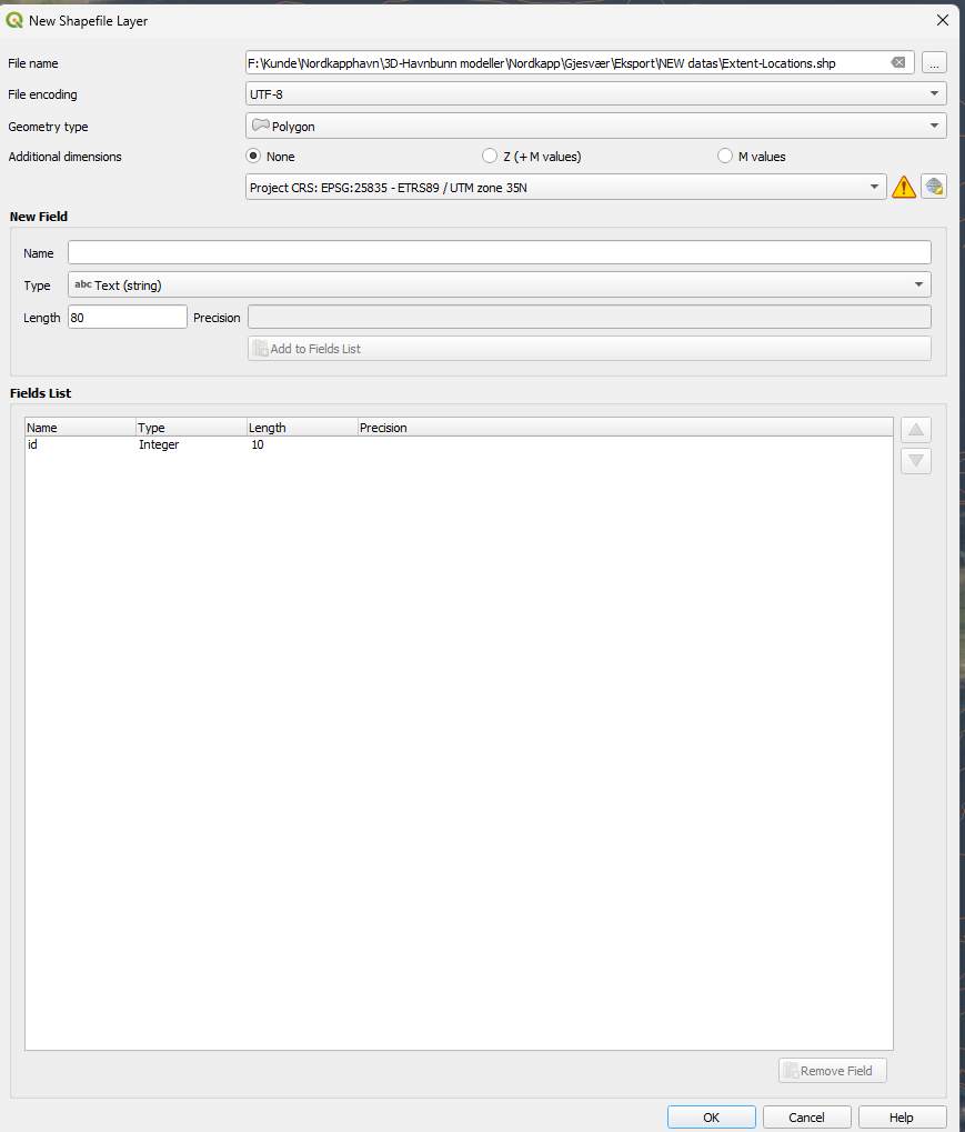
Click OK.
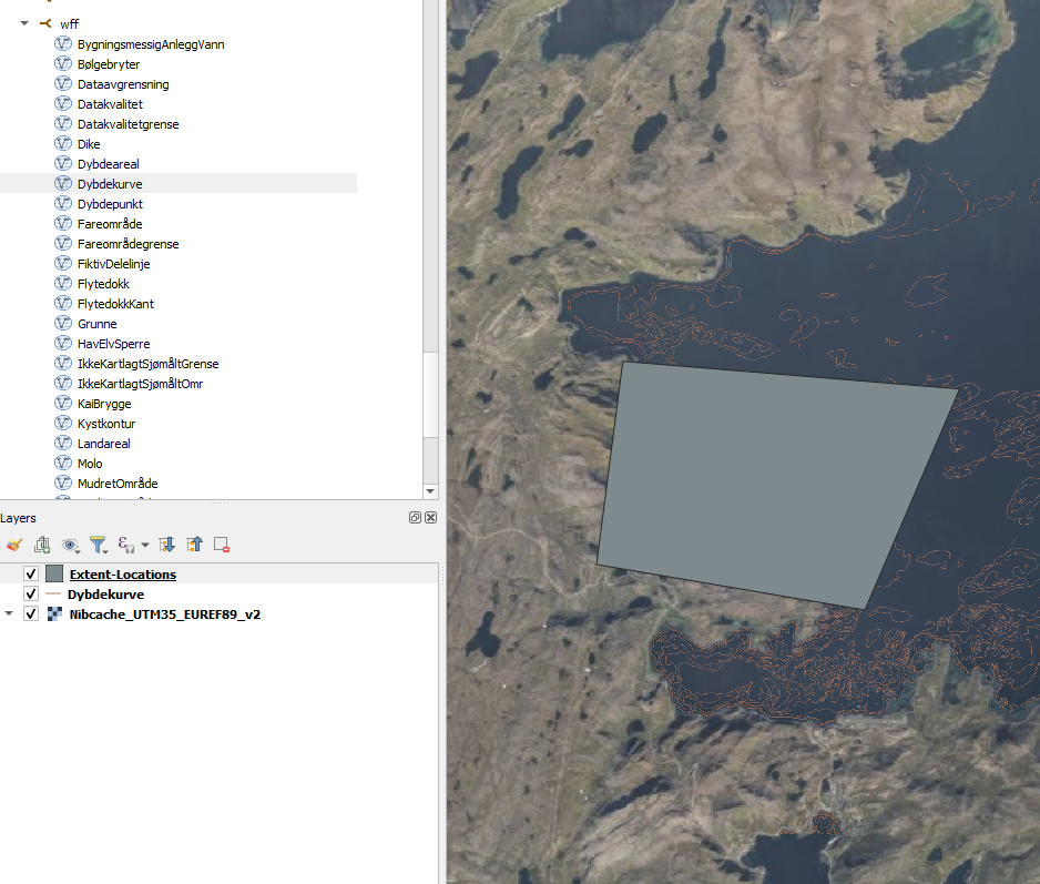
Draw Working Area
- Select the new shapefile layer
- Enable Toggle Editing (pencil icon)
- Select Add Polygon Feature
- Draw the boundary covering your project location
- Save edits
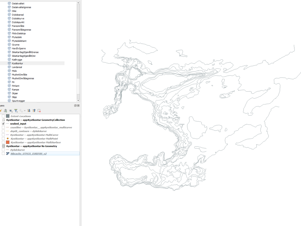
Step 2 — Load Bathymetry Contours
Add Dybdekurve from the Kartverket / Geonorge WFS service.
Processing should always be performed on locally stored data, not directly from WFS services.

Export Contours Locally
Right-click the layer → Export → Save Features As
Settings:
- Format: GeoPackage
- CRS: EPSG:25835
- Filename: “depth_contours.gpkg“
- Export field:
<em>dybde</em> - Geometry type: Automatic
- Enable Include Z-dimension
- Extent: Working polygon (Step 1)
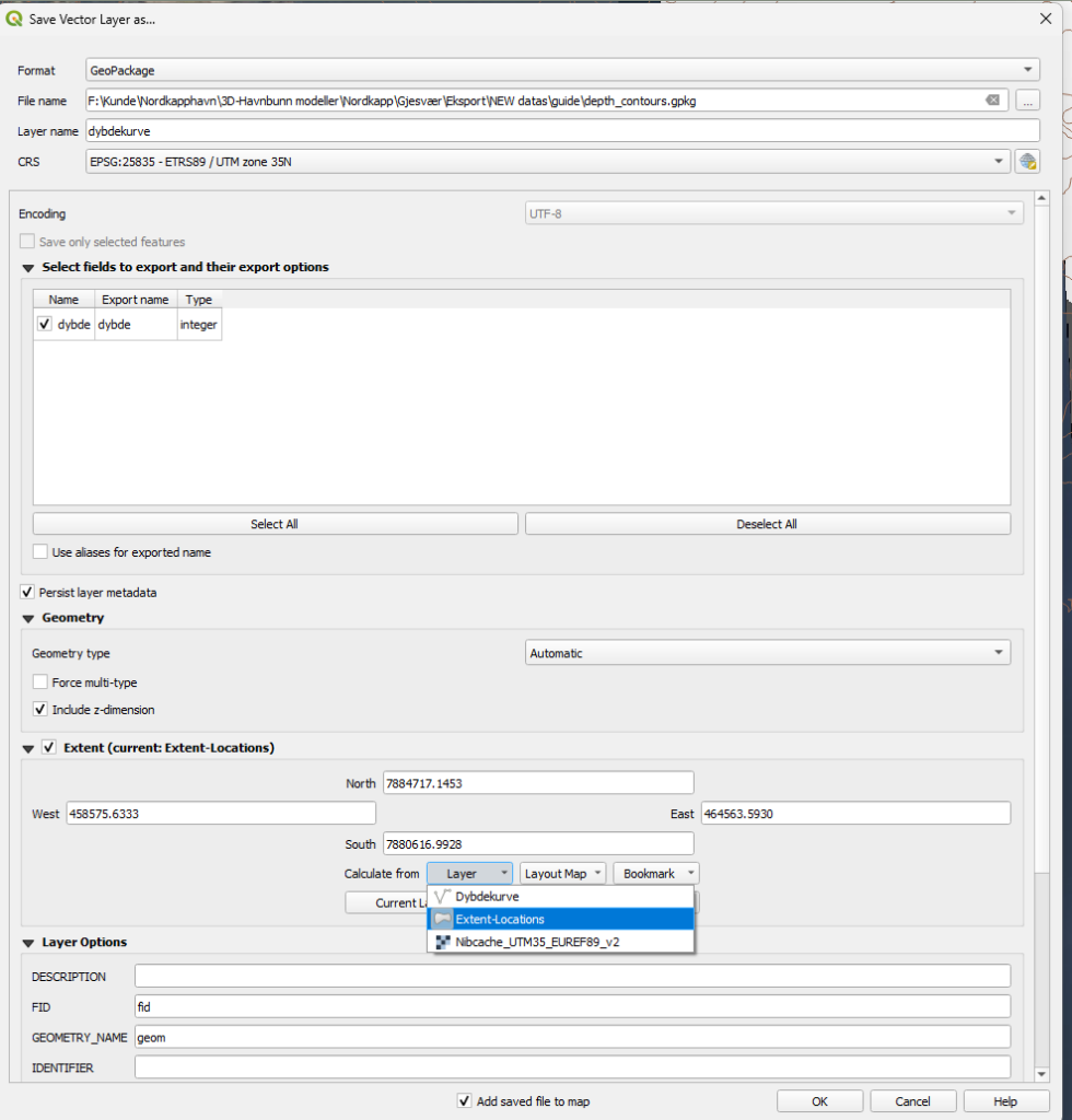
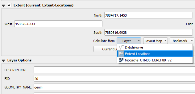
Click OK.
Step 3 — Convert Depth to Seabed Elevation
Bathymetry values represent depth below sea level and must be converted to negative elevation values.
Right Click Layer: depth_contours — dybdekurve,
Attribute Table → Field Calculator
Create new field:
- Name:
depth_neg - Type: Decimal number (real)
Expression:
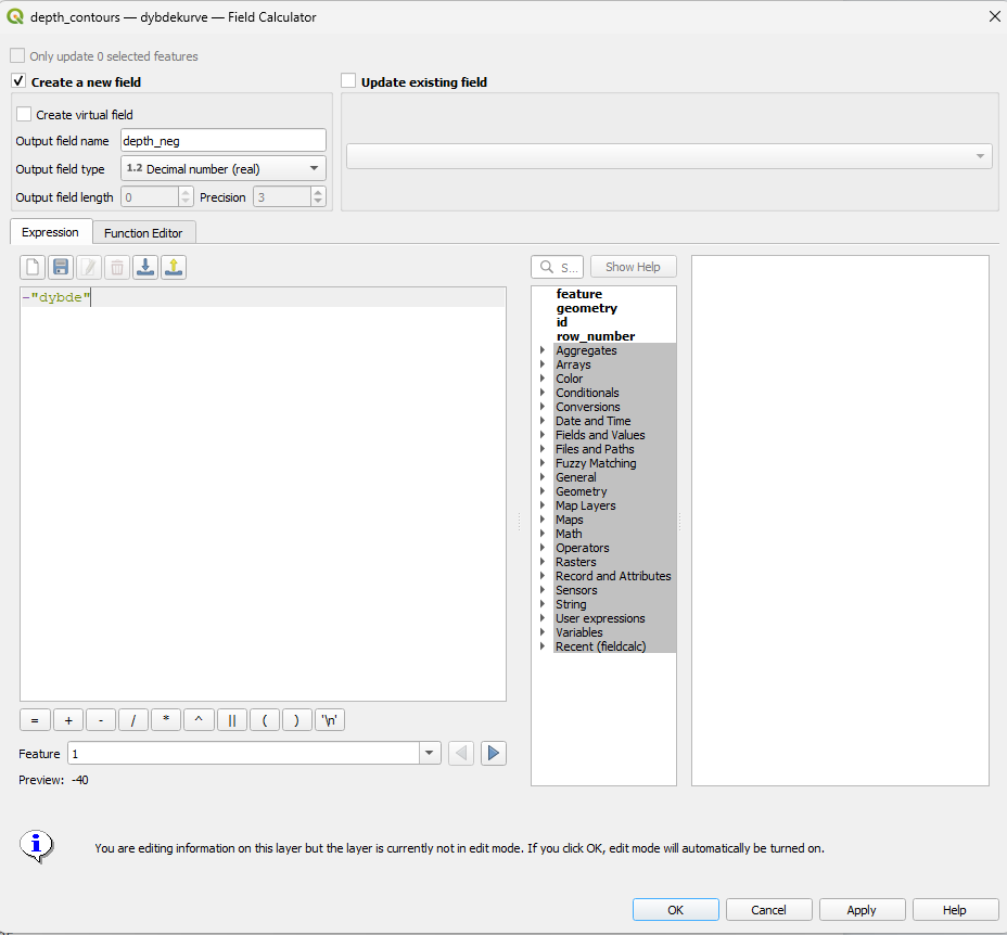
Click OK, then enable editing and Save, or (CTRL + E).
Step 4 — Add Coastline Constraint
The coastline defines sea level during interpolation.
Add Kystkontur from the same WFS service.
Export Coastline
Right-click coastline layer → Save Features As
- Format: GeoPackage
- CRS: EPSG:25835
- Filename: coastline.gpkg
- Extent: Working polygon
Click OK.
Assign Sea Level
Open Attribute Table → Field Calculator
Create field:
- Name:
depth_neg - Type: Decimal number
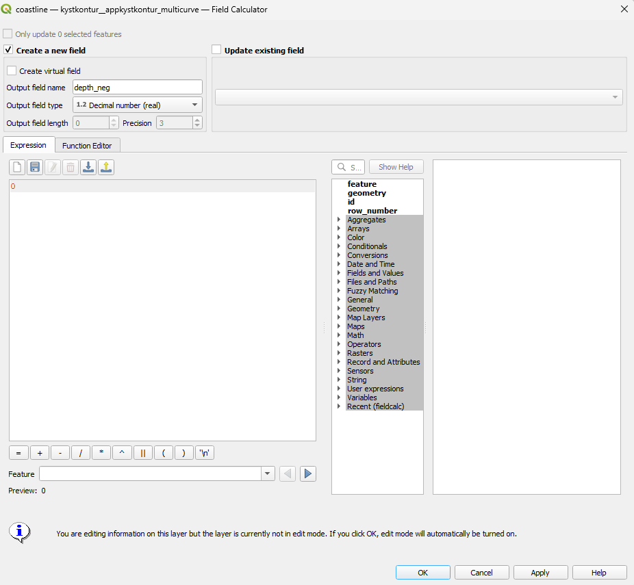
Expression:
Click OK → Save edits (or CTRL + E)
Step 5 — Merge Input Layers
TIN interpolation requires a single elevation dataset.
Open:
Processing Toolbox → Merge Vector Layers
Input:
- depth_contours
- coastline
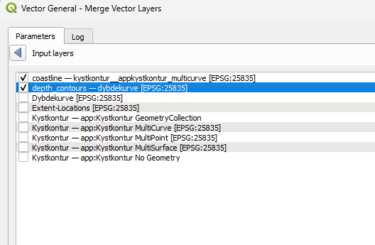
- Output: seabed_input.gpkg
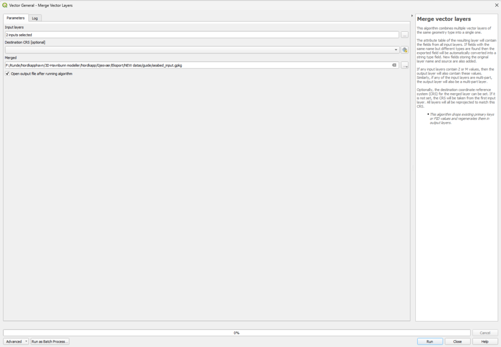
Click: Run.
Result
Step 6 — TIN Interpolation (Core Process)
Open:
Processing Toolbox → TIN Interpolation
Settings:
- Vector layer:
seabed_input - Attribute:
depth_neg - Type: Structure lines
- Method: Linear
Set Working Extent
Limit interpolation to the project polygon (Step 1).
Pixel Size
Output Raster
Save as: heightmap_interpolations.tif
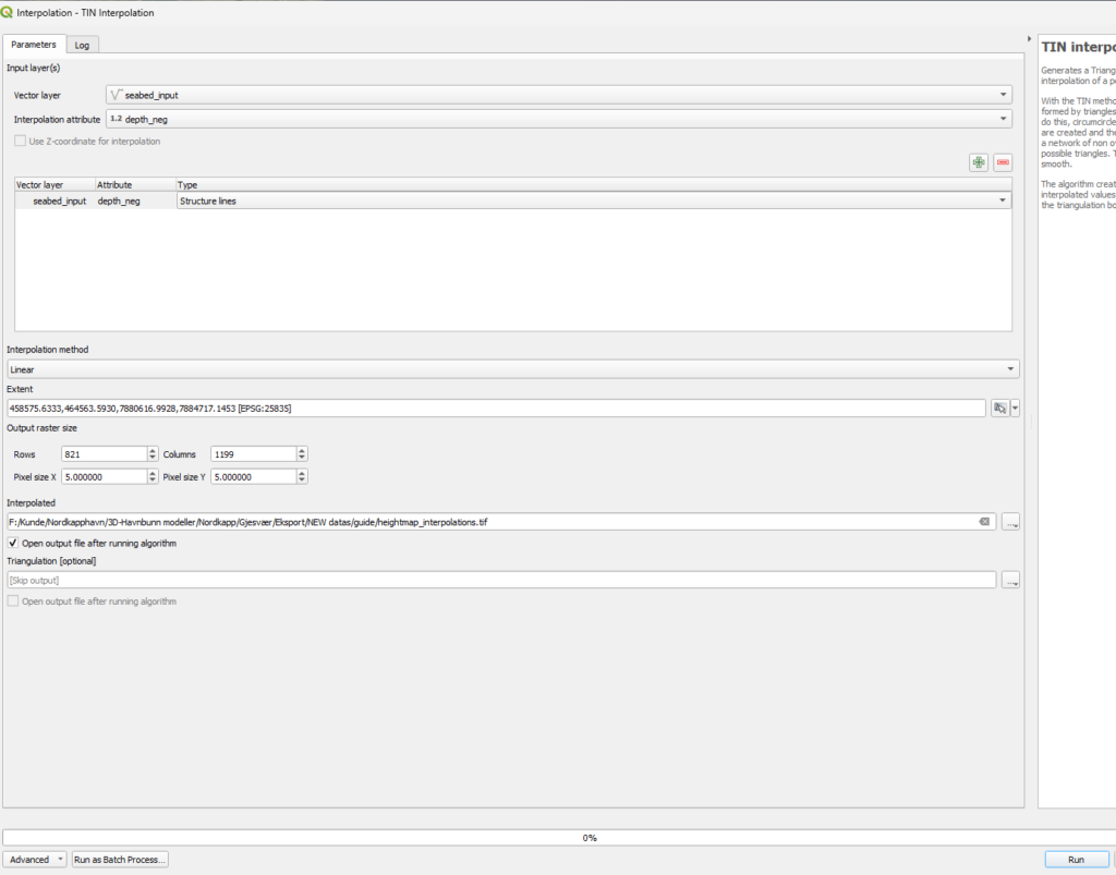
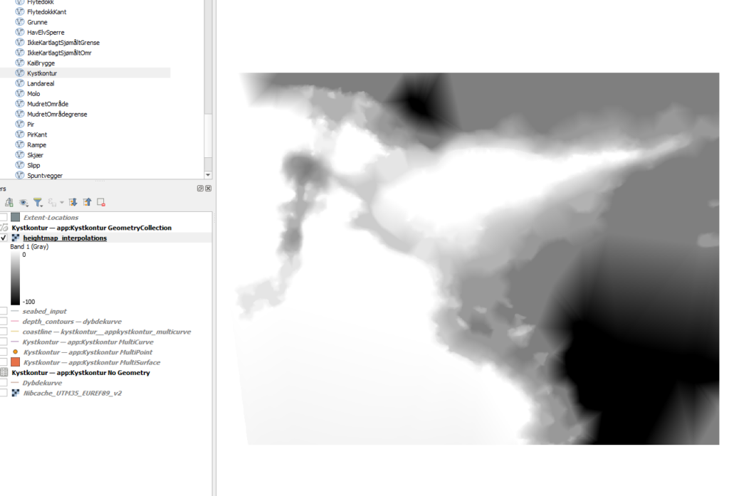
Click: Run.
The result is a continuous seabed elevation model.
Step 7 — Optional: Prepare Heightmap for Blender
For displacement workflows in Blender (none BlenderGIS), normalize elevation values.
Open:
Raster → Raster Calculator
Expression:
Output: seabed_normalized.tif
Workflow Overview
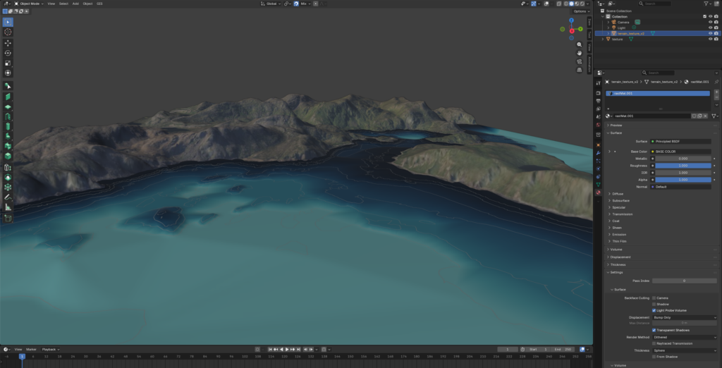
Final Result
The generated DEM provides a realistic representation of seabed morphology suitable for:
- Harbour visualization
- Planning discussions
- Digital twin environments
- Concept presentations
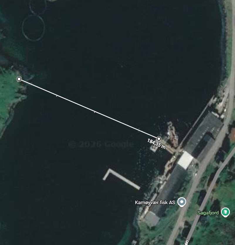
Matching the 3D Model to Real World Scale
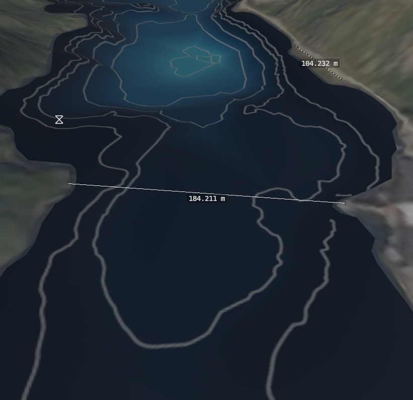
Final Thoughts
Creating a 3D bathymetry model from contour data provides a practical way to better understand underwater terrain without requiring specialized survey software or complex processing pipelines.
By combining publicly available bathymetric datasets with QGIS interpolation tools, seabed morphology can be transformed into a continuous 3D surface suitable for visualization, planning discussions, and digital twin environments.
While the workflow focuses on visualization rather than operational accuracy, it enables stakeholders to quickly interpret spatial relationships below sea level — supporting communication, concept development, and early-stage analysis.
The resulting GeoTIFF DEM or normalized heightmap can be integrated into visualization platforms such as Blender, web-based 3D viewers, or interactive harbour environments to provide intuitive insight into seabed conditions.
As digital infrastructure and port environments increasingly move toward 3D and real-time visualization, workflows like this help bridge the gap between geospatial data and accessible visual understanding.
